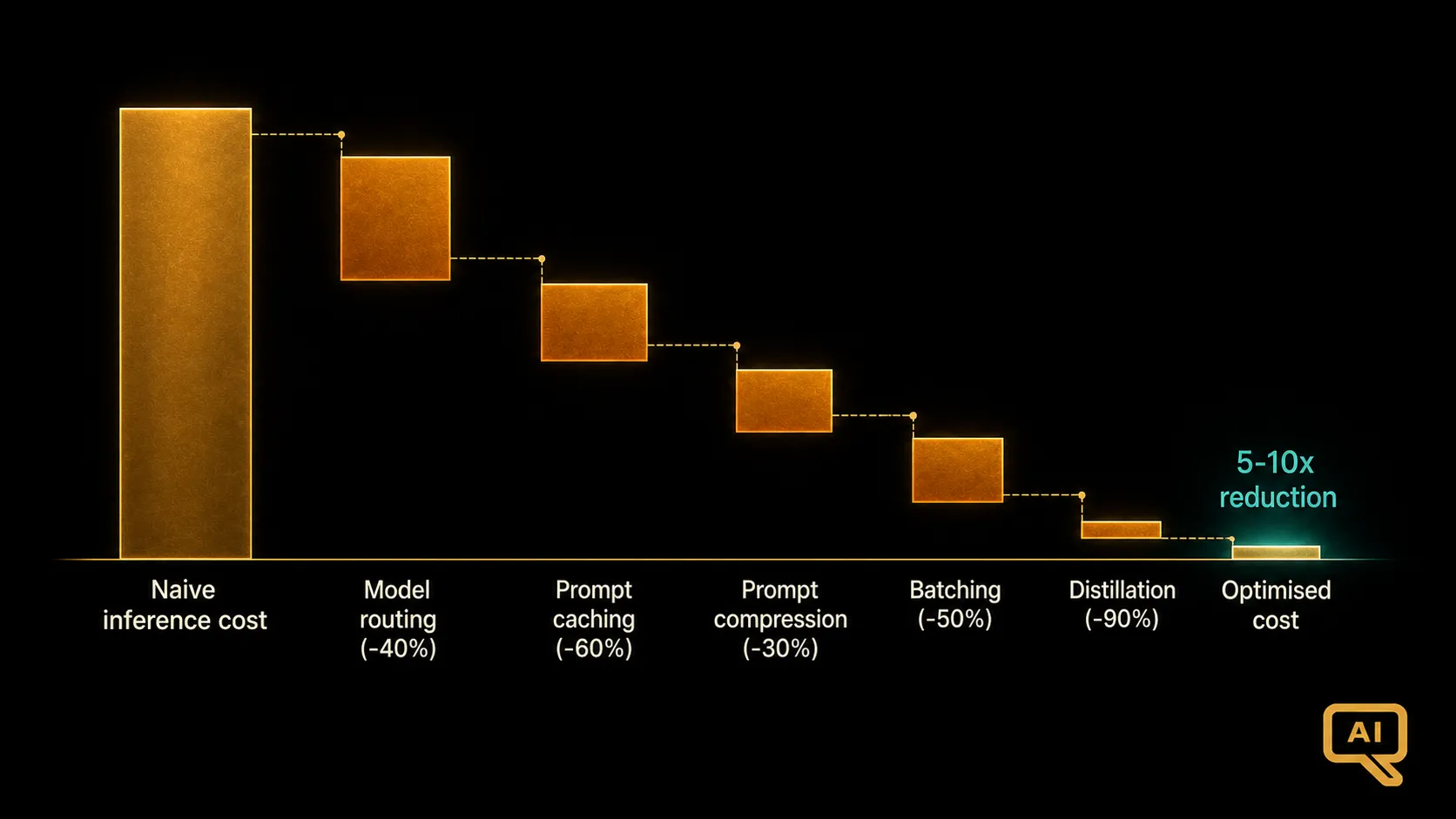
Inference is the recurring cost of AI. Training happens once (or not at all if you are using hosted models). Inference happens every time a user asks a question, every time an agent takes a step, every time a batch job runs. And unlike most enterprise software, inference costs are usage-linked in a way that scales directly with how successful the deployment is: the more people use the tool, the higher the bill.
This creates a peculiar dynamic. The organisations getting the most value from AI often have the biggest inference bills, and the organisations with tightly controlled inference spend often have the least adoption. The trick is not to minimise inference cost. The trick is to make the cost per unit of value low enough that scaling is a feature, not a threat.
That is the shift from “cost per token” to “cost per successful task” thinking, and it is where the four levers I want to walk through in this article come in.
Why the raw pricing conversation misses the point
The AI industry loves to talk about per-token pricing. As of mid-2026, Claude Haiku 4.5 is $1 per million input tokens and $5 per million output tokens; Sonnet 4.6 is $3 and $15; Opus 4.7 and 4.8 are $5 and $25. GPT-5.4 is $2.50 and $15. Grok is dramatically cheaper. Gemini Flash sits between. The pricing tables are updated weekly, and every provider is trying to shift you to their latest tier.
Focus on those numbers exclusively and you will miss the actual cost drivers. What determines your inference bill is not the sticker price. It is: the model tier you use for each request, whether you cache repeated context, how efficiently you compress prompts, whether you batch when latency allows, and how many tokens the model actually generates to complete each task. The pricing table is one input. The other four levers can each move the bill by 30 to 90 percent, and stacking them can compress cost by 10 times or more.
Lever one: model routing
The single largest cost lever in most deployments is model routing. Not every request needs the frontier model. A simple classification task can run on a small, cheap model at a fraction of the cost of the flagship. A complex multi-step reasoning task genuinely benefits from the flagship. Everything in between sits on a spectrum.
The cost differential is enormous. Sonnet 4.6 at $3/$15 versus Haiku 4.5 at $1/$5 is a 3 to 5 times difference for tasks Haiku can handle well. Opus 4.7 versus Sonnet is a similar spread. Grok Fast at $0.20/$0.50 versus Sonnet is a 10 to 30 times spread. Route intelligently and the cost impact is transformative.
The routing decision can be static (this request type always goes to this model) or dynamic (a lightweight classifier decides which model handles each request). Static routing is easier to implement and reason about. Dynamic routing captures more value but adds engineering complexity and creates a new place for the system to be wrong.
The failure mode to avoid is defaulting everything to the flagship model “just in case.” I see this constantly in early deployments. The team ships on Opus or GPT-5.5 because it works, and the token bill is manageable at low volume. Then adoption grows, the bill grows with it, and someone in finance asks whether every request really needs the flagship. The answer is almost always no, but by then the routing work is a retrofit rather than a design choice.
Lever two: prompt caching
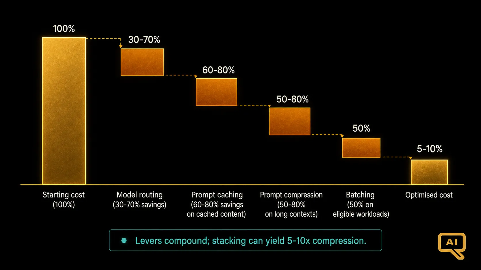
Figure 1 shows the four levers as a waterfall, which is roughly the order I would apply them in a new deployment.
Prompt caching, the second bar in Figure 1, is the next lever. Modern AI systems reuse a lot of context: system prompts, tool definitions, few-shot examples, retrieved documents, conversation history. Every one of those repeated tokens costs money each time you send them, unless you cache.
Anthropic’s prompt caching, for example, offers cache reads at 10 percent of the base input token cost, which is a 90 percent discount on cached content. For a system with a 5,000-token system prompt and 3,000-token tool definitions, caching those on every request can drop input costs by 60 to 80 percent depending on the ratio of cached to fresh content.
The catch is that caching only helps if your prompts are structured to have long stable prefixes. A system that regenerates the prompt from scratch each turn cannot cache anything. Restructuring prompts to be cache-friendly is often the single highest-leverage engineering task in an early cost optimisation pass.
Semantic caching (caching the responses to semantically similar queries, not just literal prompt matches) is a separate technique that can save 30 to 60 percent additional cost in high-repetition workloads like customer support, but it requires careful tuning of similarity thresholds to avoid returning the wrong cached answer to a slightly different question.
Lever three: prompt compression and context management
Long context is a double-edged sword. The 1 million token context window in Claude Sonnet 4.6 and later is genuinely useful for certain workloads, but every token in that context is billed on every generation step. A 100,000-token conversation history costs 10 times more per turn than a 10,000-token history, and the model’s attention is spread thinner across the additional context.
Prompt compression means using techniques (summarisation of older conversation, retrieval instead of full inclusion, structured extraction of just the relevant parts) to keep the working context small. For long-running conversations, applying a rolling summarisation strategy can cut per-turn cost by 50 to 80 percent while preserving effective continuity.
The reasoning-token dynamic is worth noting here. Modern reasoning models can generate 10 to 100 times more internal thinking tokens than they output, and those tokens are billed. A short-answer task on a reasoning model can quietly cost more than the equivalent task on a non-reasoning model despite lower per-token pricing. Effort controls on models like Claude Opus 4.8 (which lets you cap reasoning at low, high, xhigh, or max) are the operational lever for this.
Lever four: batching
The Batch API from most providers offers a 50 percent discount on both input and output tokens in exchange for asynchronous processing with a longer turnaround. For workloads where latency does not matter (overnight report generation, bulk classification, evaluation runs, data enrichment) this is essentially free money.
The failure mode is running these workloads through the synchronous API because that is what the initial implementation used. Migrating batch-tolerant workloads to the Batch API is often a two-week engineering task that saves 30 to 50 percent of the total inference bill on those pipelines.
The multiplier: distillation and small models
Beyond the four levers, there is a fifth technique that changes the economics more fundamentally: distilling capability into smaller specialised models for high-volume workloads. If you have a well-defined task that runs at millions of requests a day (classification, extraction, routing, first-pass response) you can often train or fine-tune a small model (7B to 27B parameters) to hit acceptable quality on that specific task at a fraction of the frontier model cost.
The math is dramatic. Frontier-model inference at $3 to $15 per million tokens versus a self-hosted distilled 27B model at $0.10 to $0.30 per million equivalent tokens is a 30 to 100 times cost differential. For a workload doing 10 million requests a day at 1,000 tokens per request, that is the difference between a $30,000 monthly bill and a $3,000 monthly bill.
The catch, as always, is engineering complexity. Distillation requires training data, evaluation infrastructure, self-hosting capability, and ongoing model management. It is worth it for high-volume, well-defined tasks. It is not worth it for the exploratory or low-volume paths where the frontier model’s flexibility is the point.
Cost per successful task, not cost per token
The most important shift in how I think about inference economics is moving from cost per token to cost per successful task. A cheaper model that fails half the time and requires retry with a more expensive one is not cheaper. A caching strategy that returns wrong answers 5 percent of the time is not saving money. An agentic loop that takes 20 steps to complete a task that a well-designed single-shot prompt would handle in one call is not efficient just because each step is cheap.
The right metric is total cost, including retries and failures, divided by number of successfully completed tasks. Instrumenting for this requires you to define what a successful task looks like (which is usually easier said than done, and connects back to the eval infrastructure in BCR-04), but once you have it, the optimisation conversation becomes much clearer.
Agentic AI has made this even more urgent. A multi-step agent that makes 15 model calls to complete a workflow can cost 20 to 50 times more per completed task than a single-call approach, and if the agent fails and retries the whole workflow, the cost multiplies further. Gartner’s projection that 40 percent of agentic AI projects will be cancelled by 2027 is largely driven by cost per successful task rather than by pure per-token spend.
The observability prerequisite
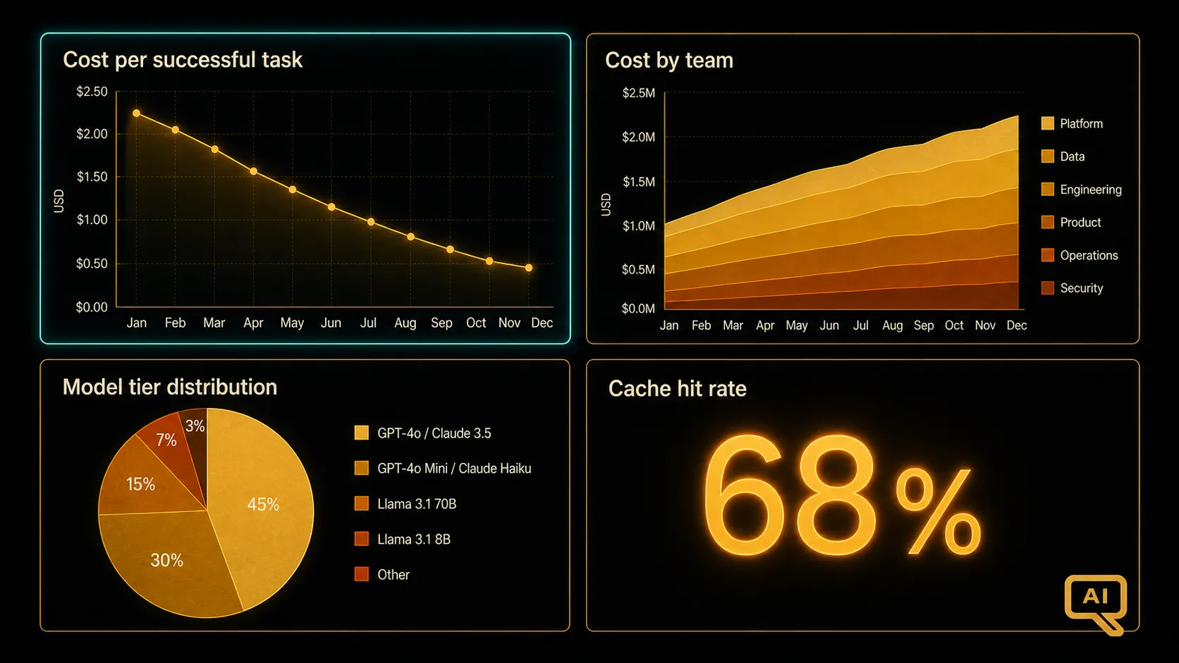
Figure 2 sketches the kind of observability layer that makes cost optimisation actually possible. Without it, you are guessing. The dashboard needs to show cost per successful task by use case, cache hit rates, model tier distribution, average tokens per request, and trends over time. It needs to break down by team or feature so you can identify where cost is growing fastest.
The four panels in Figure 2 are the minimum viable observability layer for any AI cost programme. The FinOps discipline for AI, which I cover in more depth in BCR-15, starts with this observability. Everything else is downstream of being able to see where the money is actually going.
The stacking rule
The four levers compound. A single lever might save 30 to 70 percent. Stacked correctly (routing plus caching plus compression plus batching, with distillation on high-volume paths) they can compress total inference cost by 5 to 10 times without loss of quality.
The engineering effort to get there is real, but the leverage is enormous. For any AI deployment approaching serious scale, the difference between a well-optimised inference stack and a naive one is the difference between a project finance is happy to grow and a project finance is trying to cap. Getting this right is one of the most consequential decisions in the whole AI programme, and it is one of the easiest to defer past the point where it becomes hard to fix.