
If you’ve built even a small RAG system and asked me for the single upgrade with the best return on effort, my honest answer would be re-ranking. It’s often the fastest way to turn a wobbly RAG system into a reliably good one. And the idea behind it is charmingly simple: don’t ask one method to do two jobs it’s bad at doing together. Split the retrieval into two stages, each doing what it’s best at, and the whole thing gets sharper.
This article is about that two-stage idea, why it works so well, and how to add it to your pipeline without much fuss.
The problem re-ranking solves
Semantic search over embeddings is wonderful, but it has a limitation worth naming. Embedding-based retrieval is optimised to be fast over huge collections. That speed comes at the cost of a bit of precision: it’s very good at finding chunks that are broadly on-topic, and only pretty good at telling the truly best chunk apart from the merely relevant ones.
You’ve probably seen this yourself. You inspect the top five retrieved chunks (using the habit from a couple of articles back) and think, “these are all sort of about the question, but chunk number four is the one that actually contains the answer, and it should have been ranked first.” The right material was in your top-k, just not in the right order. If you had only used top-3 that day, the truly best chunk would have been cut off.
That mismatch between broadly relevant and precisely best is what re-ranking exists to fix.
The two-stage idea
Re-ranking splits retrieval into two stages that do complementary jobs. Figure 1 shows the shape.
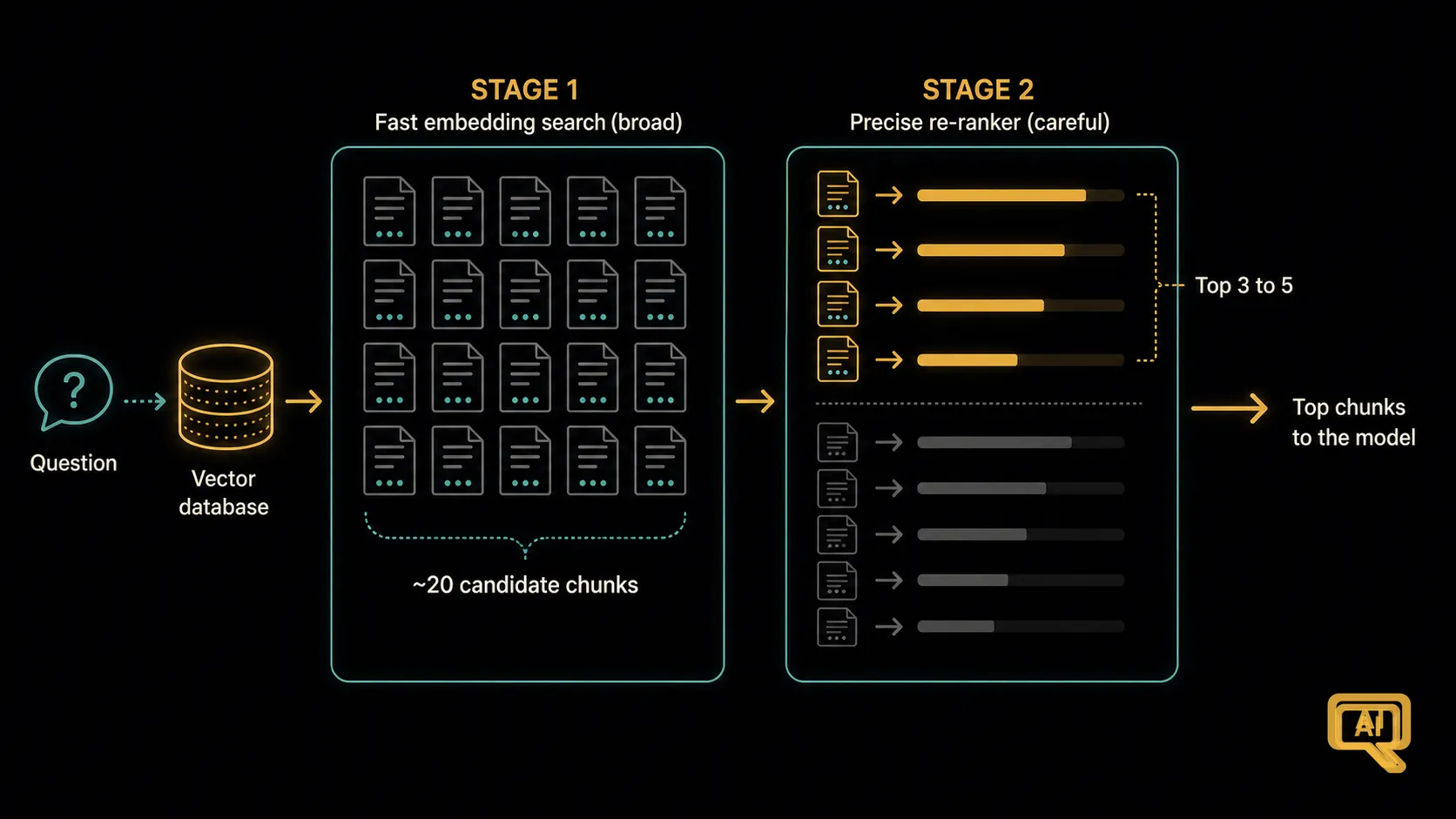 Figure 1: Stage 1 uses fast embedding search to fetch a broad set of candidate chunks. Stage 2 uses a slower, more precise re-ranker to re-order those candidates and keep only the truly best few for the model.
Stage one is what you already have: a fast embedding search that pulls a broad set of candidates. Instead of grabbing your usual top-5, you deliberately grab more, maybe the top-20 or top-30. The goal at this stage is recall: cast a wide-enough net that the truly best chunk is somewhere in there, even if it isn’t at the top.
Stage two is the new part: a re-ranker takes those 20 candidates and re-orders them, this time using a more careful, more accurate scoring method. Because it only has to look at 20 chunks (not millions), it can afford to be slower and smarter. From its re-ranked list, you keep just the top few, say 3 to 5, and hand those to the language model.
The result is a small, sharp set of chunks that beats what plain embedding search would have produced on its own. Nothing about your documents, your chunking, or your embeddings has to change. You’ve just added a second, more discerning pass at the end.
What actually does the re-ranking?
The re-ranker is usually a specialised model, and the important thing to know about it is why it does better than the first pass, not exactly how it works inside.
Embedding search compares two vectors: the question’s vector against each chunk’s vector. Fast, but it’s judging them “at arm’s length,” through a single geometric distance. A re-ranker, by contrast, looks at the question and each candidate chunk together, examining how the words in the question actually relate to the words in the chunk. It’s slower (which is why we don’t use it on the whole collection), but it can spot subtler matches that embeddings alone miss. The technical name you’ll bump into for this kind of model is a cross-encoder, and if you’re browsing tools you’ll see names like Cohere Rerank or open-source options such as bge-reranker. You don’t need to memorise them, just recognise that a re-ranker is a proven, off-the-shelf component; you don’t build one, you plug one in.
In pseudocode, adding re-ranking looks like this:
# Stage 1: fast embedding search, grab a broad set
candidates = vector_db.search(query_embedding=q_emb, top_k=25)

# Stage 2: re-ranker scores each candidate against the question, precisely
scores = reranker.score(question, [c.text for c in candidates])

# Keep the top 3-5 for the model
top = sort_by_score(candidates, scores)[:5]
That’s it. A handful of lines, and retrieval quality typically jumps.
Why this is such a big win
Look at what the two stages are doing. The first cares mostly about recall: getting the right chunk into the candidate set at all. The second cares mostly about precision: putting the truly best chunk on top. Neither method is good at doing both jobs alone. Together they cover each other’s weaknesses. Figure 2 shows how the ranking often shifts between the two stages.
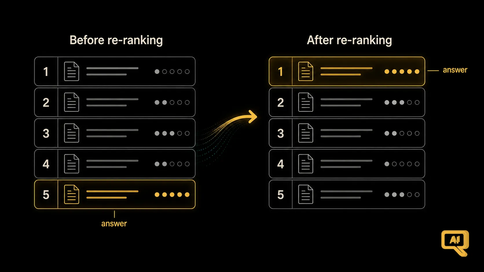 Figure 2: The candidate set from stage 1 has the answer in it, but perhaps ranked fifth. After re-ranking, the truly best chunk rises to the top and the shakier candidates drop away. Same starting set, dramatically better final ranking.
This is why re-ranking so reliably pays off. You’re not asking your embedding model to be smarter; you’re asking a second, better-suited judge to take a careful look at a shortlist. It’s the natural human process of shortlist-then-decide, translated into your pipeline.
The trade-offs to know about
Nothing is free. Re-ranking has three costs worth being honest about, though all are usually well worth paying:
- Slower. You’re doing a second pass, and the re-ranker is slower per item than a similarity lookup. In practice this is often just tens of milliseconds on a shortlist of 20 to 30 chunks, but it’s not zero.
- More work per query. You’re calling an extra model (or an extra service), which adds a bit of infrastructure and, if it’s a paid API, a small extra cost per query.
- Slightly more moving parts. Something else to configure, monitor, and pay for. Not a lot more, but worth acknowledging.
Given how much the quality tends to improve, these costs are usually a bargain, especially for use cases where a wrong answer is expensive. But it’s a real trade-off, so make it consciously.
Where re-ranking fits in your journey
Here’s the practical advice I’d offer. Get the basics right first: good chunking, sensible top-k, a clean grounded prompt. Then, if you find that the right chunk is often in your retrieved set but not at the top (a diagnosis the “look at what was retrieved” habit will surface quickly), add re-ranking. It’s a well-understood upgrade with a big pay-off and a small amount of new complexity. There’s a reason nearly every mature RAG system uses it.
If you want a mental picture: think of re-ranking as promoting your retrieval process from a fast, generalist first-round sift to a fast first-round plus a careful second-round decision. You wouldn’t hire from a stack of one thousand résumés without shortlisting first; you also wouldn’t shortlist without then carefully reading the top handful. RAG works the same way, and re-ranking is that second read.
We’ve now made the retrieval step precise. Next, we look at making it broader. Semantic search can occasionally miss things that a good old keyword search would have caught easily, and combining both is a small change that solves a very real class of misses. That’s hybrid search, and it’s next.
Next in the series: Hybrid Search: Semantic + Keyword, combining meaning-based and word-based search to catch what each misses on its own.