
In the last article we drew the whole RAG pipeline, and the query phase had a line in it that looked deceptively simple: search the vector database and get the top matches. It read like one atomic step. It isn’t. That single line hides a small cluster of choices — how many chunks to fetch, what “similar” actually means, and whether you should be searching your whole collection at all — and getting those choices right is one of the easiest, cheapest ways to make a RAG system noticeably better.
This article opens up the retrieval step and shows you the three main knobs you have on it: the similarity measure, the top-k you fetch, and metadata filtering. None of them are complicated, but they’re often the difference between average and excellent retrieval.
Knob 1: How “similar” is defined
The whole idea of semantic search is finding the passages closest to your question in meaning-space. But what exactly does “closest” mean, mathematically? Vector databases give you a choice — and the most common one, and the one you should reach for by default, is cosine similarity.
Cosine similarity ignores how long two vectors are and only cares whether they point in the same direction. Two passages that go on for very different lengths but are about the same thing point the same way — so cosine similarity says they’re similar, which is exactly what we want. It focuses purely on meaning, not length.
You’ll occasionally see other options — Euclidean distance (straight-line distance in space) or dot product (a similar idea to cosine, but sensitive to length). For nearly all RAG work, cosine is the sensible default. It’s what most embedding models are designed for, and unless you have a specific reason to pick something else, don’t. You don’t need to master the maths — just know the choice exists, know it’s usually made for you, and know that cosine similarity is the standard for RAG.
Knob 2: Top-k — how many chunks to fetch
Top-k is the number of best-matching chunks you retrieve for each question — the “top k” results. It’s a single number, but its effect is surprisingly big.
- Set it too low (say, 1 or 2), and you might miss important context. If the answer needs facts from two different chunks, and you only grabbed one, the model will answer poorly.
- Set it too high (say, 30 or 50), and you flood the prompt with irrelevant text. The signal gets buried, costs go up, and the model can lose focus on the passages that actually matter.
Figure 1 shows this Goldilocks pattern.
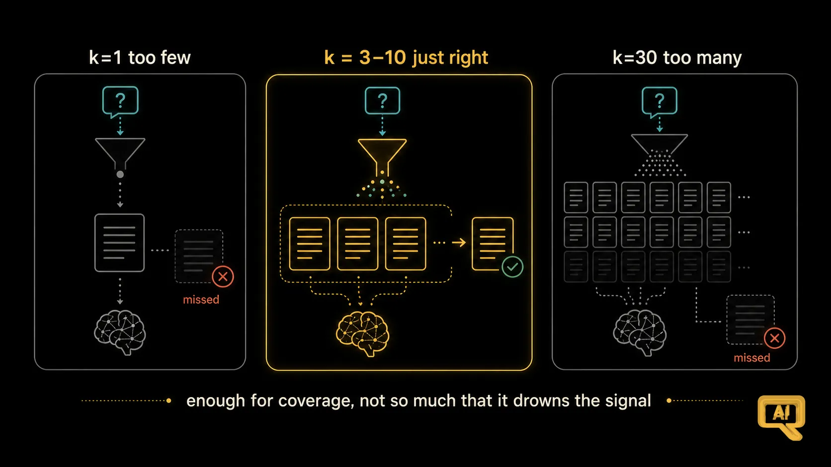 Figure 1: Too few chunks retrieved and you miss context needed to answer. Too many and you drown the model in irrelevant material. The sweet spot fetches enough for coverage without diluting the signal.
For most RAG systems, a good starting range is somewhere between 3 and 10. That’s usually enough to give the model what it needs without cluttering the prompt. As with chunk size, the exact right number depends on your content and your questions — and it’s worth trying a few values and looking at the results.
There’s a subtle refinement worth knowing about too. Some systems set a similarity threshold as well: “only include chunks whose similarity score is above X.” This is useful because it means when nothing is a good match, you retrieve nothing — and the model then honestly says “I couldn’t find that in the documents” instead of trying to answer from a mediocre chunk. Combining top-k with a threshold (“up to 10 chunks, but only if similarity ≥ 0.7”) is a lovely little upgrade.
Knob 3: Metadata filtering — search less to search better
Here’s the knob people underuse the most, and it’s often the highest-value one of all. Every chunk you store can carry metadata — the source file, the section it came from, its date, tags you care about. Recall that we recommended storing this metadata back in the chunking article. Now it earns its keep.
Metadata filtering means restricting your search to the chunks that meet certain criteria before similarity is computed. Only the refund policy document. Only chunks written after 2024. Only chunks tagged as “public.” The vector database then searches purely within that subset. Figure 2 shows why this makes such a difference.
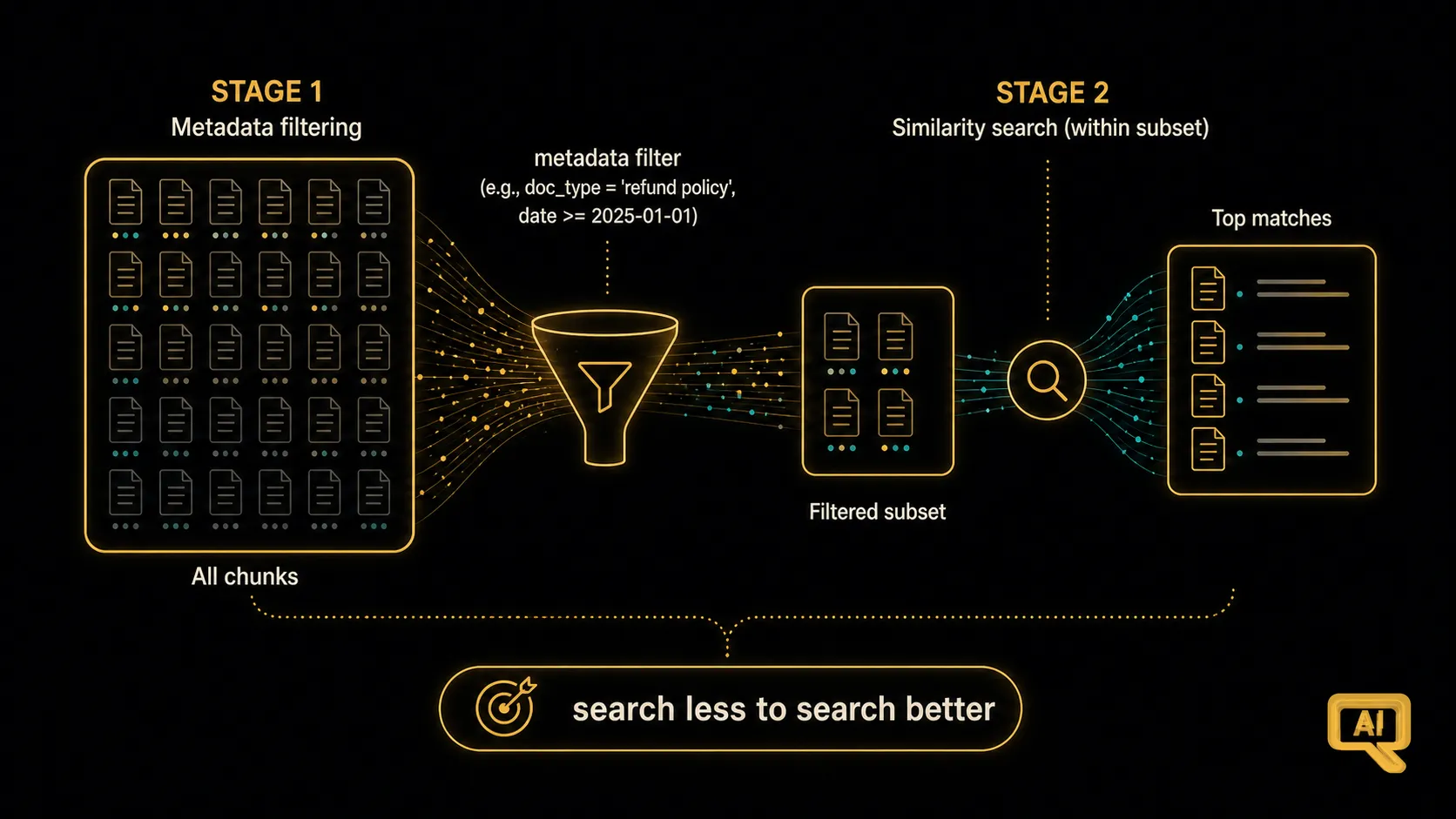 Figure 2: Metadata filtering narrows the collection first — say, to just the refund policy — and only then runs the similarity search. You get more accurate matches and cheaper searches, because the database ignores everything irrelevant to the question up front.
Why is this so powerful? Two reasons. First, it dramatically improves precision — the search can no longer accidentally return a beautifully similar but irrelevant chunk from the wrong document. Second, it makes searches faster and often cheaper, because there’s less material to search through in the first place. And a hidden third benefit: when your user’s question implies a scope (“in the 2026 pricing sheet, what does the enterprise tier cost?”), filtering lets you honour that scope explicitly, instead of hoping semantic similarity will figure it out.
Simple metadata filters that pay off almost immediately include: document type, section or category, date, language, and access-level (only search what this user is allowed to see). In pseudocode, using it looks like this:
results = vector_db.search(
    query_embedding=q_emb,
    top_k=5,
    filters={"doc_type": "policy", "date": {"$gte": "2025-01-01"}}
)
The database handles both the filter and the similarity search efficiently in one shot.
Where the metadata should come from
For all this to work, someone (or something) has to attach useful metadata during ingestion. This is another reason to invest in that ingestion phase — the more you learn about each chunk when you first import it, the more you can filter later. Some sensible defaults to capture for every chunk:
- Source — the file, URL, or system it came from
- Structural location — the section, chapter, or page
- Date — when the document was created or last updated
- Type — policy, FAQ, transcript, marketing, and so on
- Any tags meaningful to your domain
Two minutes of thought here saves hours of retrieval headaches later.
A quick recap of your retrieval toolkit
You now have three knobs on the retrieval step:
- Similarity measure — leave it on cosine unless you have a strong reason not to.
- Top-k (and optionally a threshold) — usually a small number, 3 to 10, tuned by looking at real results.
- Metadata filtering — the underused superpower that narrows the search to what’s actually relevant.
Put all three together, and you get retrieval that’s not only more accurate but also faster and cheaper — a rare trifecta.
When retrieval works and when it doesn’t
Even with these knobs turned well, RAG systems will sometimes give bad answers. The really valuable question is: when a bad answer comes back, was it a problem in retrieval or somewhere else? This is the debugging question that separates people who build RAG systems from people who fix them — and it’s exactly what the next article is about. It’s the piece already up on the site: why your RAG pipeline keeps hallucinating, and how to diagnose which stage is actually to blame.
Next in the series: Why Your RAG Pipeline Keeps Hallucinating — diagnosing which step is really failing when the answers go wrong.