A Practical Guide to Fine-Tuning an Open Model

Time to move from theory to something you could actually run. This article is a practical guide to fine-tuning an open model with LoRA, end to end. It’s not a copy-paste-and-forget tutorial, because the exact commands change with every library version, but it is the honest map of the real steps, the real decisions, and the real gotchas, in the order they’ll show up. By the end you should feel like you know how to actually do this, not just talk about it.

I’ll write the code snippets in a widely-used, readable style so they make sense even if you never run them. If you do run them, use them as a scaffold and consult the current documentation of your chosen library for the small details.

The high-level plan

Every LoRA fine-tuning job follows the same shape. Six steps, in order, shown in Figure 1.

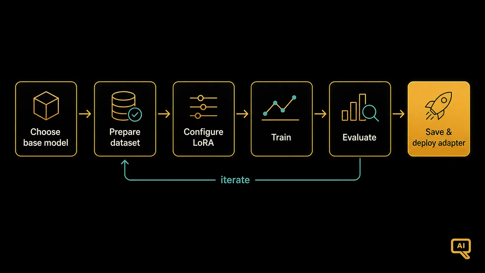Figure 1: The workflow. Pick a base model, prepare your dataset, configure LoRA, run training, evaluate the result, and save the adapter for deployment. Each step is small; together they get you from data to a working fine-tuned model.

Let’s walk through each step.

Step 1: Choose a base model

Your first real decision is which open model to fine-tune from. A few practical points:

• Match the model size to your task and hardware. For most style and format tuning, models in the roughly 7 to 13 billion parameter range are the sweet spot: capable, fine-tunable on modest hardware with QLoRA, and cheap to run. Anything much larger and hosting starts to hurt; anything much smaller and quality suffers.
• Prefer instruction-tuned models over pure base models for most business tasks. An “instruct” or “chat” variant already knows how to follow instructions; fine-tuning it into your style is a much smaller lift than starting from a raw base model. Look for names with “-Instruct” or “-Chat” suffixes.
• Check the license. Some open models are freely usable commercially; others have restrictions. Choose one that matches your intended use.
• Popular starting points as of writing include the Llama, Mistral, Qwen, and Gemma families. Pick a recent, well-supported release of one of these and you’ll be in good shape.

Once you’ve picked, load it in your training script:

from transformers import AutoModelForCausalLM, AutoTokenizer

model_name = "meta-llama/Llama-3.1-8B-Instruct"   # example, adjust to your choice
tokenizer = AutoTokenizer.from_pretrained(model_name)
model     = AutoModelForCausalLM.from_pretrained(model_name)

Nothing fancy yet. Just loading the base model and its matching tokenizer.

Step 2: Prepare your dataset

If you followed the dataset article, you already have a clean set of high-quality input-and-output pairs. Now you need to load them into the training script and format them the way the model expects during training.

Most modern training tools want the examples in a chat format, structured like a small conversation:

from datasets import Dataset

# Your prepared examples as a list of dicts
raw = [
    {"input":  "My order arrived damaged.",
     "output": "I'm sorry your order arrived that way. Please reply with a photo..."},
    # ... more examples ...
]

def to_chat(ex):
    return {"messages": [
        {"role": "user",      "content": ex["input"]},
        {"role": "assistant", "content": ex["output"]},
    ]}

dataset = Dataset.from_list([to_chat(ex) for ex in raw])
train_ds, eval_ds = dataset.train_test_split(test_size=0.1).values()

A few things worth noticing. First, we split off a small evaluation slice (say 10%) that we do not train on. Second, the exact format the tokenizer expects may differ slightly by model family, so consult the model’s docs for the correct chat template. This is one of the mundane details that will bite you if you skip it.

Step 3: Configure LoRA

Now the LoRA piece. The library peft (parameter-efficient fine-tuning, remember from the last article) is the standard way to set this up:

from peft import LoraConfig, get_peft_model

lora_config = LoraConfig(
    r=16,                       # size of the LoRA adapter, common values: 8, 16, 32
    lora_alpha=32,              # a scaling factor, often 2x r
    lora_dropout=0.05,          # small dropout for regularisation
    bias="none",
    task_type="CAUSAL_LM",
    target_modules=["q_proj", "k_proj", "v_proj", "o_proj"],   # attention layers
)

model = get_peft_model(model, lora_config)
model.print_trainable_parameters()
# -> e.g. "trainable params: 33M / total params: 8B (0.4%)"

Two things worth understanding here. r controls how big the LoRA adapter is; higher r means a bigger adapter with more capacity, but also more to train. Start with 16 for most tasks. And target_modules picks which layers get the adapters; the attention projections (the q_proj, k_proj, v_proj, o_proj shown) are the standard, most effective choice. The print_trainable_parameters() line prints how many parameters you’re actually training, and seeing a number like 0.4% is the moment LoRA feels real.

If you’re memory-constrained, this is where you’d add QLoRA by loading the base model in a quantised form:

from transformers import BitsAndBytesConfig
import torch

quant = BitsAndBytesConfig(
    load_in_4bit=True,
    bnb_4bit_quant_type="nf4",
    bnb_4bit_compute_dtype=torch.bfloat16,
)
model = AutoModelForCausalLM.from_pretrained(model_name, quantization_config=quant)

Load it in 4-bit like this, then apply the LoRA config on top. That’s QLoRA in three lines.

Step 4: Train

Now the training loop itself. The trl library (transformer reinforcement learning, which also handles supervised fine-tuning) gives you a wrapper that keeps this short:

from trl import SFTTrainer, SFTConfig

config = SFTConfig(
    output_dir="./ft-output",
    num_train_epochs=3,           # 2-3 is often enough for LoRA
    per_device_train_batch_size=4,
    gradient_accumulation_steps=4, # effective batch size = 4 * 4 = 16
    learning_rate=2e-4,           # a common LoRA learning rate
    logging_steps=25,
    eval_strategy="steps",
    eval_steps=100,
    save_steps=200,
)

trainer = SFTTrainer(
    model=model,
    args=config,
    train_dataset=train_ds,
    eval_dataset=eval_ds,
    tokenizer=tokenizer,
)

trainer.train()

A few hyperparameters to know about, since these are the ones you’ll actually tweak:

• num_train_epochs is how many times the trainer walks through your entire dataset. For LoRA on style/format tasks, 2 or 3 epochs is usually enough. More often causes the model to overfit and lose general ability.
• learning_rate controls how big each nudge is. LoRA tolerates a higher learning rate than full fine-tuning; something in the 1e-4 to 3e-4 range is a good starting point.
• batch_size and gradient_accumulation_steps together set your effective batch size. Bigger is more stable but needs more memory; the accumulation trick lets you simulate a bigger batch on smaller hardware.

During training, watch the evaluation loss on your held-out slice. If it stops improving or starts rising while training loss keeps falling, you’re starting to overfit. Stop early.

Step 5: Evaluate what you got

Training is done. Now the honest question: is the fine-tuned model actually better? Do this before you deploy anything, because a fine-tune that feels better on the first three examples you try is often not the fine-tune that is better across your real use cases. Figure 2 lays out a sensible evaluation approach.

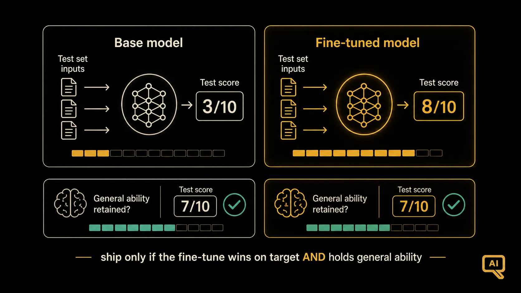Figure 2: Compare the fine-tuned model against the base model on a held-out test set. Score both on your task’s real quality criteria and check that general ability hasn’t regressed. Only ship if the fine-tune wins on both.

Two things to check, one obvious and one easily forgotten:

• On the task you fine-tuned for, does it clearly beat the base model? Run the same test set through both, score the results (either by eye against clear criteria, or with the model-as-judge trick from the earlier evaluation article), and compare. If the fine-tune isn’t clearly better, either your data or your setup needs work.
• Has general ability held up? Test the fine-tuned model on a few tasks outside your fine-tuning domain, questions it should still handle competently. If it’s noticeably worse than the base on general things, you may have over-trained (too many epochs, or too small a learning rate saved for too long). This is the “catastrophic forgetting” trap from earlier articles.

Only ship if both boxes tick.

Step 6: Save and deploy the adapter

The useful thing about LoRA is what you save is tiny: just the adapter weights, usually a few tens of megabytes, not the whole model. This makes distribution and versioning much simpler.

model.save_pretrained("./my-tuned-adapter")
tokenizer.save_pretrained("./my-tuned-adapter")

To use the adapter at inference time, you load the base model and then apply the adapter on top:

from peft import PeftModel

base = AutoModelForCausalLM.from_pretrained(model_name)
tuned = PeftModel.from_pretrained(base, "./my-tuned-adapter")

And now tuned behaves according to what you fine-tuned. That’s the whole path from raw data to a deployable fine-tuned model.

Practical realities I want you to know about

A few things worth internalising before you dive in.

• Your first run will not be your final run. Expect to iterate on the dataset, hyperparameters, and evaluation criteria a few times. Don’t book a big compute slot for run one.
• Most fine-tuning problems are dataset problems in disguise. If the results are underwhelming, look at your data before you look at your hyperparameters.
• Start small on cheap hardware to shake out bugs, then scale up when the pipeline is working end to end. There is nothing more painful than discovering a data-formatting bug three hours into an expensive training run.
• Version everything: the dataset, the training config, and the resulting adapter. When someone (probably future you) asks “which version of the adapter produced this behaviour?”, the answer needs to be a single command away.
• Log carefully. Training loss, evaluation loss, and sample generations at regular intervals. Numbers on their own are misleading; seeing a few sample outputs from the model every few hundred steps is what actually tells you if it’s learning what you wanted.

From doing to steering

You now have a working end-to-end mental model for how to actually fine-tune an open model with LoRA. The mechanics are clear. But so far we’ve focused on the supervised style of fine-tuning, showing the model good input-output pairs and having it copy them. There’s a related family of techniques that goes further: teaching a model to follow instructions in general, and shaping its behaviour toward what humans actually prefer. That’s the world of instruction tuning and RLHF, and it’s where we head next.

---

Next in the series: Instruction Tuning & RLHF Explained, how models are aligned to be helpful.