How Networks Learn: Loss, Gradient Descent & Backpropagation

We’ve said it several times now: a neural network “learns” by adjusting its weights until its outputs match the examples. I’ve been asking you to take that on faith. Now I want to pay off the promise and show you how that actually happens, because it’s the training loop everything else depends on, and it’s more intuitive than it sounds.

Picture the challenge honestly. A network can have millions of weights, all starting out as random numbers, all producing nonsense. Somehow the machine has to figure out which way to nudge every single one of those millions of dials to make its answers a little less wrong, and then do it again, and again, thousands of times. How does it know which way to turn each knob? The answer comes in three parts.

Part 1: Loss: putting a number on “how wrong”

Before you can fix a mistake, you need to measure it. In machine learning, that measurement is called the loss: a single number that says how wrong the network’s prediction was. Small loss means “close to right.” Big loss means “way off.” The entire goal of training is to make the loss as small as possible.

The simplest version is just the gap between the prediction and the truth. If the right answer was 90 and the network guessed 75, it was off by 15. We usually square that gap (so that being off by a lot is penalised much more than being off by a little, and so negatives don’t cancel positives):

def loss(prediction, actual):
    return (prediction - actual) ** 2

print(loss(75, 90))   # 225  -> quite wrong
print(loss(88, 90))   # 4    -> much closer

That’s it. Loss is just a wrongness score. Now the whole problem of learning becomes a single clear mission: find the weights that make this number as small as possible.

Part 2: Gradient descent: moving downhill

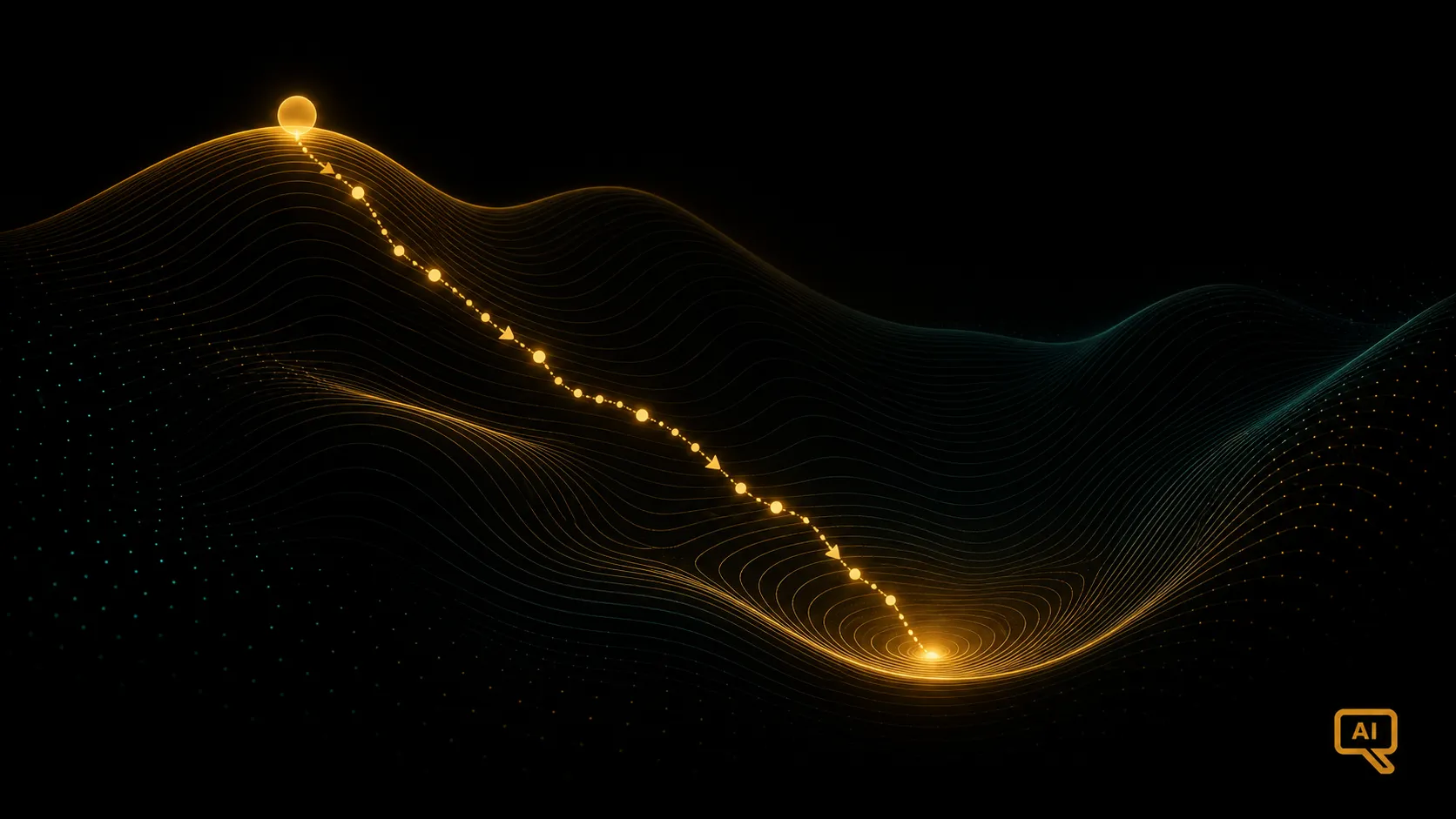
Here’s the idea for how to shrink the loss. Imagine every possible combination of the network’s weights laid out as a vast surface of hills and valleys, where the height at any point is the loss for those weights. High ground is bad (lots of error); low valleys are good (little error). Training is the search for the lowest valley.

Now imagine you’re standing somewhere on this surface in thick fog. You can’t see the whole map, only the ground right under your feet. How do you get lower? You feel which way the ground slopes downward, and you take a step that way. Then you feel again, and step again. Keep going, and you’ll wind your way down into a valley. Figure 1 captures this picture.

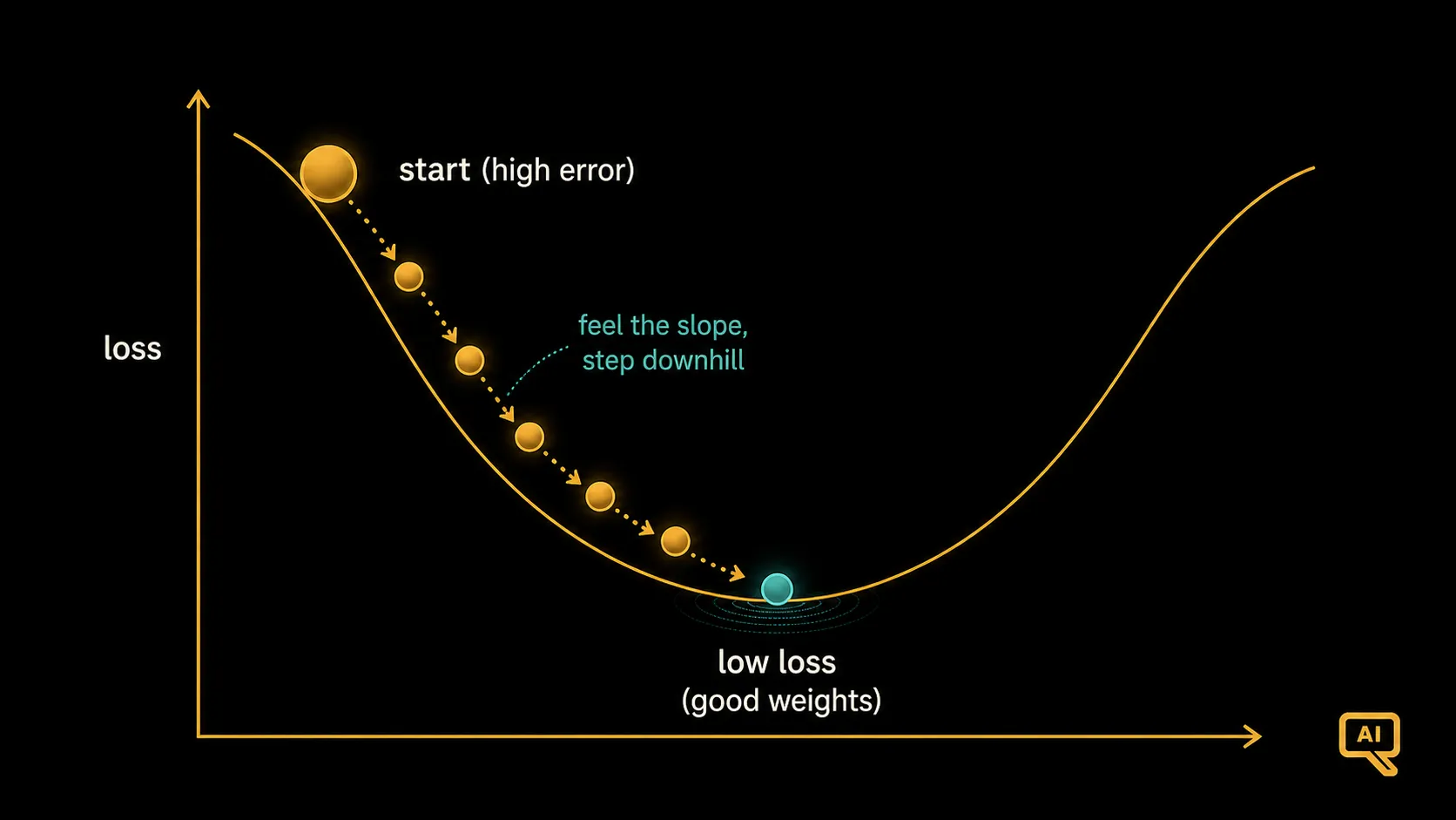Figure 1: The loss surface. Starting high (lots of error), the network feels the slope beneath it and steps downhill again and again, settling toward a valley where the loss is low.

This method is called gradient descent, and the fancy word “gradient” just means slope: which way, and how steeply, the ground falls away. The recipe is:

1. Check the slope of the loss with respect to a weight (which way is downhill?).
2. Nudge the weight a small step in the downhill direction.
3. Repeat, over and over.

The size of each step has a name too: the learning rate. Big steps get you down faster but risk bounding right over the valley; tiny steps are safe but slow. Choosing it well is part of the craft.

In one line of maths, each update is: new weight = old weight − (learning rate × slope). The minus sign is the trick: we move against the slope, i.e. downhill.

Here’s gradient descent shrinking the error on a single weight, so you can watch it work:

# Goal: learn the weight w so that w * 2 gets close to the target, 10. (Answer: w = 5)
w = 0.0                 # start with a random guess
learning_rate = 0.1
x, target = 2.0, 10.0

for step in range(20):
    prediction = w * x
    error = prediction - target
    slope = 2 * error * x          # which way the loss changes if we nudge w
    w = w - learning_rate * slope  # step downhill
print(round(w, 2))                 # ~5.0  -> it found the right weight on its own

Starting from a random guess of zero, the weight moves toward 5, the value that makes the prediction correct. Nobody told it the answer. It just kept stepping downhill on the loss. Scale this up to millions of weights, and you have the essence of how every neural network learns.

Part 3: Backpropagation: sharing out the blame

Gradient descent needs to know the slope for every weight, which way to nudge each one. In a deep network with many layers, that’s the tricky part. When the final answer is wrong, which of the millions of weights, buried across all those layers, was responsible, and by how much?

The method that answers this is backpropagation (usually shortened to “backprop”). The idea is to work backwards. You start at the output, where you can directly see the error, and you pass the blame back through the network layer by layer. Each layer figures out how much it contributed to the mistake, then hands the appropriate share of blame to the layer before it. Figure 2 shows this two-way flow.

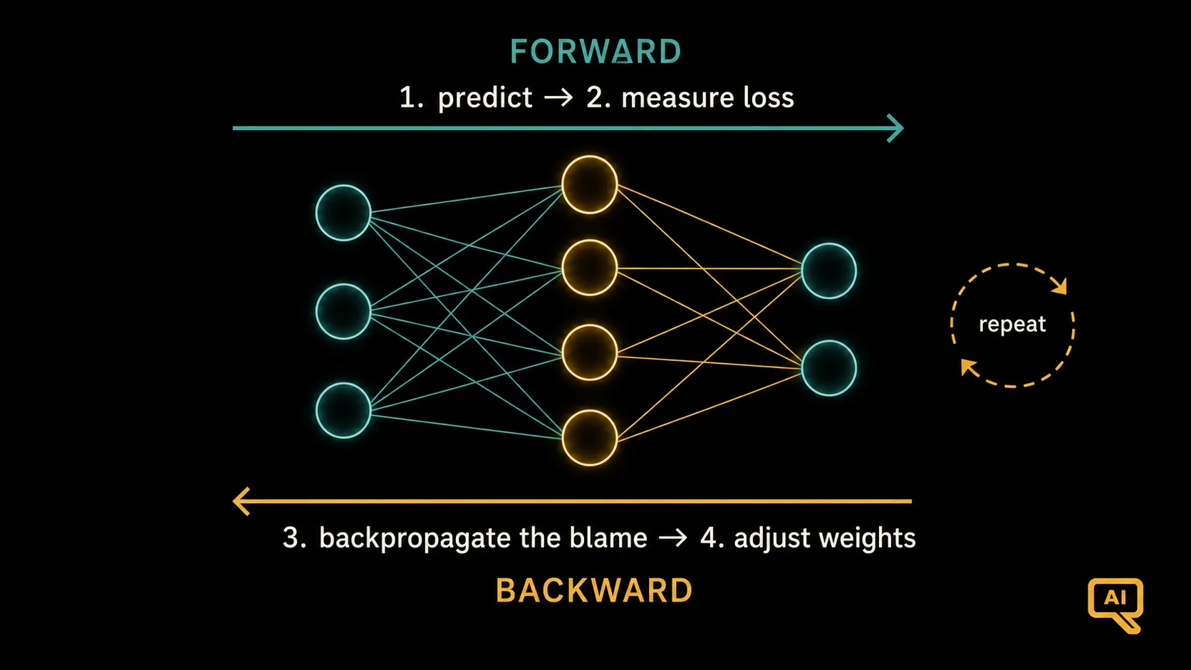Figure 2: Information flows forward to make a prediction and compute the loss. Then the blame flows backward through the layers, backpropagation, so every weight learns which way to nudge. Then the whole loop repeats.

I find an analogy helps here. Imagine a company ships a faulty product and traces the fault back through the assembly line: the final inspector pinpoints the defect, then works backwards asking each station how much it contributed, so each one knows exactly what to fix. Backprop does the same, assigning each weight its fair share of responsibility for the error, so gradient descent knows which way to nudge every single one.

Put the three parts together and you have the full learning loop, shown in Figure 2:

1. Forward: feed in an example, let the network make a prediction.
2. Measure: compute the loss: how wrong was it?
3. Backward: use backpropagation to find each weight’s share of the blame.
4. Adjust: nudge every weight a small step downhill (gradient descent).
5. Repeat: millions of times, across millions of examples.

The training loop

When I step back, this is the part that still amazes me. There’s no magic, no hand-coded intelligence. Just a wrongness score, a slope to follow downhill, and a clever way of sharing out the blame, repeated relentlessly. Do that enough times on enough data, and a pile of random numbers gradually organises itself into weights that can recognise a face, translate a language, or, as we’re building toward, model the patterns of human language.

Much of modern AI rests on this loop. But there’s still a gap between what we’ve built and a system that understands language, and it has to do with sequences: in a sentence, order and context are everything, and the networks we’ve described so far handle inputs one fixed chunk at a time. Closing that gap is the story of the next few articles, starting with an early, clever, but ultimately limited idea for handling sequences.

---

Next in the series: Sequence Models & Why RNNs Struggled: the first attempt to give networks a memory for language.